NumPy에 대해 알아보자. ③
Array Operation
Elementwise operations
In [1]:
import numpy as np
a = np.array([1, 2, 3, 4])
a
Out[1]:
In [2]:
a + 1
Out[2]:
array를 거듭제곱으로도 넣을 수 있다.
$$ [2^1, 2^2, 2^3, 2^4] $$In [3]:
2**a
Out[3]:
In [4]:
b = np.ones(4) + 1
b
Out[4]:
In [5]:
a - b
Out[5]:
In [6]:
a + b
Out[6]:
In [7]:
c = np.ones((3, 3))
c
Out[7]:
In [8]:
# element-wise, NOT Matrix product
## 매트릭스의 곱이 아니라. 원소간의 곱이다.
c * c
Out[8]:
In [9]:
# matrix product
c.dot(c)
Out[9]:
In [10]:
a = np.array([1, 2, 3, 4])
b = np.array([4, 2, 2, 4])
array끼리의 Boolean은 각 원소끼리 비교한다.
In [11]:
a == b
Out[11]:
In [12]:
a > b
Out[12]:
In [13]:
a = np.array([1, 2, 3, 4])
b = np.array([4, 2, 2, 4])
c = np.array([1, 2, 3, 4])
np.array_equal( a, b) a와 b 어레이가 같은지 확인!
In [14]:
np.array_equal(a, b)
Out[14]:
In [15]:
np.array_equal(a, c)
Out[15]:
특수 함수에 한 번에 넣을 수 있다.
In [16]:
a = np.arange(5)
a
Out[16]:
In [17]:
np.sin(a)
Out[17]:
In [18]:
np.log(a)
Out[18]:
In [19]:
np.exp(a)
Out[19]:
In [20]:
np.log10(a)
Out[20]:
In [21]:
a = np.arange(4)
b = np.array([1, 2])
a, b
Out[21]:
In [22]:
a + b
In [23]:
x = np.array([1, 2, 3, 4])
x
Out[23]:
In [24]:
np.sum(x)
Out[24]:
In [25]:
x.sum()
Out[25]:
In [26]:
x = np.array([[1, 1], [2, 2]])
x
Out[26]:
In [27]:
x.sum()
Out[27]:
In [28]:
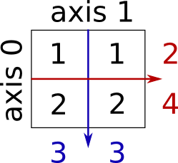
x.sum(axis=0) # columns (first dimension)
Out[28]:
In [29]:
x.sum(axis=1) # rows (second dimension)
Out[29]:
In [30]:
x = np.array([1, 3, 2])
min, max, argmin, argmax
x.argmin( )
index of minimum
x.argmax( )
index of maximum
In [31]:
x.min()
Out[31]:
In [32]:
x.max()
Out[32]:
In [33]:
x.argmin() # index of minimum
Out[33]:
In [34]:
x.argmax() # index of maximum
Out[34]:
all, any
all : 모든 것이
Trueany :
True가 하나라도 있으면True, 모든 것이False이면,False이다.
In [35]:
np.all([True, True, False])
Out[35]:
In [36]:
np.any([True, True, False])
Out[36]:
In [37]:
# 아래 dtype을 int로 지정을 해줘야, 아래서 올바른 Boolean 값을 얻을 수 있다.
a = np.zeros((100, 100), dtype=np.int)
a
Out[37]:
In [38]:
np.any(a != 0)
Out[38]:
In [39]:
np.all(a == a)
Out[39]:
In [40]:
a = np.array([1, 2, 3, 2])
b = np.array([2, 2, 3, 2])
c = np.array([6, 4, 4, 5])
In [41]:
((a <= b) & (b <= c)).all()
Out[41]:
mean, median, std, var
In [42]:
x = np.array([1, 2, 3, 1])
y = np.array([[1, 2, 3], [5, 6, 1]])
In [43]:
x.mean()
Out[43]:
In [44]:
np.median(x)
Out[44]:
In [45]:
# last axis = 마지막 axis = -1 여기서는 axis = 1 (가로)
np.median(y, axis=-1)
Out[45]:
In [46]:
x.std() # full population standard dev.
Out[46]:
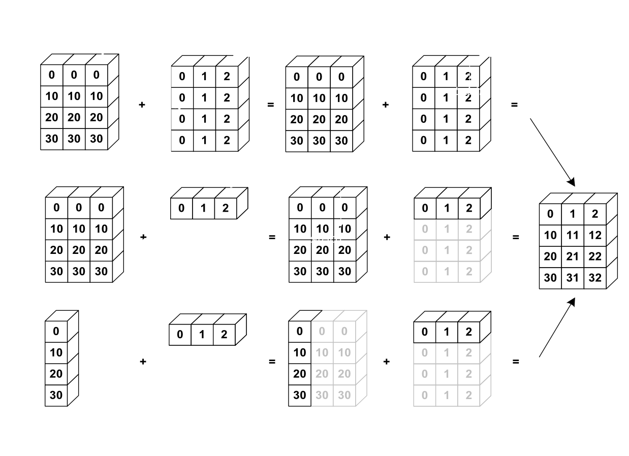
Broadcasting
In [47]:
a = np.tile(np.arange(0, 40, 10), (3, 1)).T
a
Out[47]:
In [48]:
b = np.array([0, 1, 2])
b
Out[48]:
In [49]:
a + b
Out[49]:
In [50]:
a[:,0][:, np.newaxis]
Out[50]:
In [51]:
a[:,0][:, np.newaxis] + b
Out[51]:
In [52]:
a = np.ones((4, 5))
a
Out[52]:
In [53]:
a[0]
Out[53]:
In [54]:
a[0] = 2
a
Out[54]:
In [55]:
x, y = np.arange(5), np.arange(5)[:, np.newaxis]
In [56]:
x
Out[56]:
In [57]:
y
Out[57]:
In [58]:
# 원소 각각 제곱한후, Broadcasting
distance = np.sqrt(x ** 2 + y ** 2)
distance
Out[58]:
ogrid, mgrid, meshgrid
실제로는 mgrid, meshgrid를 많이 쓴다.
shape을 서로 맞춰준다.
(가로, 세로)
3차원 그림을 그릴 때, 꼭 알아야 한다.
np.ogrid
In [59]:
x, y = np.ogrid[0:3, 0:5]
In [60]:
x
Out[60]:
In [61]:
y
Out[61]:
In [62]:
# -1 ~ 1까지 3조각으로 나눠라, 5조각으로 나눠라. j가 없으면 stack으로 인식한다.
np.ogrid[-1:1:3j, -1:1:5j]
Out[62]:
In [63]:
# j가 없으면 stack으로 인식한다.
np.ogrid[-1:1:3, -1:1:5]
Out[63]:
np.mgrid
In [64]:
# Broadcasting을 위한 차원 뻥튀기를 해준다.
x, y = np.mgrid[0:3, 0:5]
In [65]:
x
Out[65]:
In [66]:
y
Out[66]:
In [67]:
np.mgrid[-1:1:3j, -1:1:5j]
Out[67]:
In [68]:
X, Y = np.meshgrid(np.arange(3), np.arange(5))
In [69]:
X
Out[69]:
In [70]:
Y
Out[70]:
In [71]:
# ravel()는 짝 펴주는 메소드, view
## (x,y)로 점을 찍고 싶을 때 사용
a = zip(X.ravel(), Y.ravel())
list(a)
Out[71]:
중요!!
In [72]:
import matplotlib.pylab as plt
%matplotlib inline

# -1 ~ 1 까지 10개로, -2 ~ 2까지 10개로 → meshgrid로 인해 Broadcasting된 후 각각 10 by 10 array
## (가로, 세로)
a = np.meshgrid(np.linspace(-1,1,10), np.linspace(-2,2,10))

# meshgrid 결과 나오는 두 array를 아래로 쌓음.
b = np.vstack(a)

# reshape으로 처음 만들었던 array 두 개가 각각 원소가 되는 어레이로 변경함.
c = b.reshape(2,-1)

# array를 list로 변경
d = c.tolist()

# *를 붙여서 d의 list를 x, y로 인식하게 하여 산점도를 그림
plt.scatter(*d)
Out[72]:
